
Introduction
Filters are used in almost all electronic circuits for many different frequency ranges, from a few hertz to HF. A filter allows signals from one range to pass through and blocks another range. Low-pass, high-pass, and band-pass filters, as well as band-stop filters, can be generated either analogue or digital, and filters for higher frequencies can also be generated using microstrip lines, waveguides, or coaxial cables.
Since low-noise frequency response is especially desirable in the audio range, higher frequencies are filtered accordingly, thereby reducing noise. Another important example is filtering before analog-to-digital conversion as unnecessary higher frequencies can cause aliasing effects (overlapping) which in turn can increase the noise level. In HF transmission, the baseband signal is modulated onto a carrier by a mixer before transmission. In addition to unwanted mixing results, this also results in frequency images that have to be filtered before the signal is amplified and transmitted.
A well-known example is the use of the filter in telephony. In this case an analog frequency range of 300 Hz to 3400 Hz (voice) is transmitted, sampled at 8 kHz and digitized. Therefore, the audio signal that our voice carries is filtered by the telephone with a bandpass filter. It is also important to minimize aliasing effects that can arise from incorrect sampling of higher frequency components. A side effect is that not all the frequencies of the voice pass through and the voice sounds “filtered”. Another example in telephony is the splitter (divider) used in DSL technology. Here the frequency range is divided for analog or digital telephony (signaling and voice) on the one hand and for digital data for the Internet (DSL) on the other. They can then be filtered with the corresponding filter.
To be able to correctly adjust components such as filters, especially during the design phase, it is necessary to resort to measured technology as well as calculations and optimization with the appropriate software. Spectrum analyzers, such as RIGOL's DSA800 series, or Vector Network Analyzers (VNAs), such as RIGOL's RSA3000N series, can be used in high-frequency applications. However, conventional spectrum analyzers are not suited for the low frequency range as they typically have a starting frequency range of 9 kHz and the necessary tracking generator starts at 100 kHz. On the other hand, it is not possible to measure the phase in the frequency range with analyzers that use the heterodyne principle. While the second problem can be solved with a VNA, the first problem remains unresolved. However, one of the most practical tools for visualizing the transmission characteristics of a component is the Bode plot.
The Bode plot was developed in the late 1930s by Hendrik Wade Bode while working for Bell Laboratories in the US with the aim of being able to better present and evaluate work on broadband components. The graph is full log for gain and half log for phase. This means that, for gain, both the Y-axis for amplitude difference and the X-axis for frequency are displayed logarithmically. It allows you to visualize even the smallest changes over a very large frequency range. For the phase, the X axis is expressed in degrees (°). In this way not only filters but also, for example, operational amplifier circuits or control circuits can be measured.
With the MSO5000 series oscilloscopes and the Bode plot function, RIGOL offers an optimal solution to carry out these tests precisely in the lower frequency range of 10 Hz to 25 MHz. outputs of the arbitrary waveform generator (25 MHz / 200 MS/s / 14 bit) of the MSO5000. These generators also output arbitrary signals up to 16 kpts in length and incorporate many basic waveforms and various types of analog modulation. With the arbitrary function, the measured signals can be viewed on the screen, uploaded to the generator, and stored on the device for download and later analysis.
The Bode diagram is a very useful tool to show the frequency response of a circuit, for example that of a filter. On the one hand, these curves can be represented as geometric curves that contain the information about magnitude and phase. However, the display in the frequency range also serves to improve your interpretation. The change in voltage amplitude and the phase evolution can be displayed and measured in two separate curves, which can also be described as the frequency characteristic method. The MSO5000 series supplies harmonic AC signal frequencies (sinusoidal signals) from one of the two outputs of the arbitrary waveform generator. Frequencies are generated with a defined spacing between frequencies that covers a certain range of frequencies. The frequency range is displayed logarithmically to clearly show a large frequency range and give a good overview. The vertical representation of the amplitude variation (that is, the positive or negative amplification of the transformer) is expressed in dB (see formula 1).
![]()
Formula 1: Gain α (vertical axis of the Bode plot).
The phase shift is expressed (not logarithmically) in degrees (°). The output of the generator can be separated with a power splitter and is connected to analog input 1 of the oscilloscope on the one hand, and to the measurement object (eg a filter) on the other. The output of the filter is connected to analog input 2. With channel 1, channel 2 and swept sine in the frequency range of the MSO5000 generator the transfer function can now be displayed. The structure of the measure appears in the block diagram of Figure 1.

Figure 1: Measurement blocks by Bode plot with the RIGOL MSO5000 series oscilloscope.
A simple filter can be used to describe the Bode plot functions on the MSO5000 series oscilloscopes as in the example. As indicated above, a filter can block part of the frequency band and let another part through. Figure 2 shows a low pass filter as an example. It passes all frequency components from a low frequency range, eg 0 Hz up to the upper limit frequency, and blocks all higher frequency components.
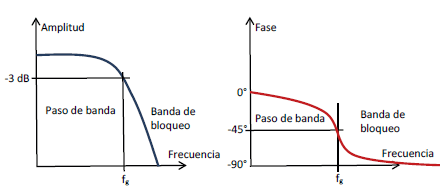
Figure 2. Phase and amplitude curves of a simple first-order low-pass filter.
Figure 2 characterizes the frequency response of the amplitude and phase curve in the frequency range of the low pass filter. This information describes the complex relationship between the filter and the frequency, which is due to the inductive and/or capacitive components of the filter. In this example, the cutoff frequency is defined by either the 3dB rolloff or the filter phase position at -45°. When designing the filter, both values can be obtained by fine-tuning passive components such as resistors, inductances, or capacitors. For example, simple RC elements can be used up to about 100 kHz. The higher frequency ranges are implemented with RLC elements, among others. These devices can also be used with active elements such as amplifiers when the output amplitude of the step will need to be higher than the input amplitude.
Mathematically it can be described as follows for a simple first-order RC low-pass filter:
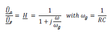
Formula 2: Transfer function of a simple first-order RC low-pass filter.
Formula 2 indicates that the filter cutoff frequency can be defined by selecting the resistance (R) and capacitance (C). The value and the angle can be calculated from formula 3, which also corresponds to the curve in figure 2:

Formula 3: Calculation of magnitude and angle for a first order low pass RC filter.
With the Bode plot you can measure different parameters. One of these parameters is the phase margin (phase margin, PM). PM describes the phase distance or phase margin from 0° to the actual measurement point at the position whose gain is 0 dB (ie the amplitude of the point has the same value as the output amplitude). In some transmission systems these parameters can be very important. For example, if the PM is very small, depending on the function, the components may assume an unwanted wobble property. The higher its value, the greater the stability. Another parameter describes the amplifier margin (amplifier margin, GM). Similar to PM, GM is a measure of relative stability. Here, with a phase position of 0°, the amplitude difference or amplitude reserve is measured at 0 dB and is automatically marked on the Bode plot and displayed as a measured value. Depending on the transmission system, it can also happen that if this value is very small, it also has the effect of an oscillator. The same is true here: the higher this value, the greater the stability. Both values appear in Figure 3 in a measurement taken as an example.
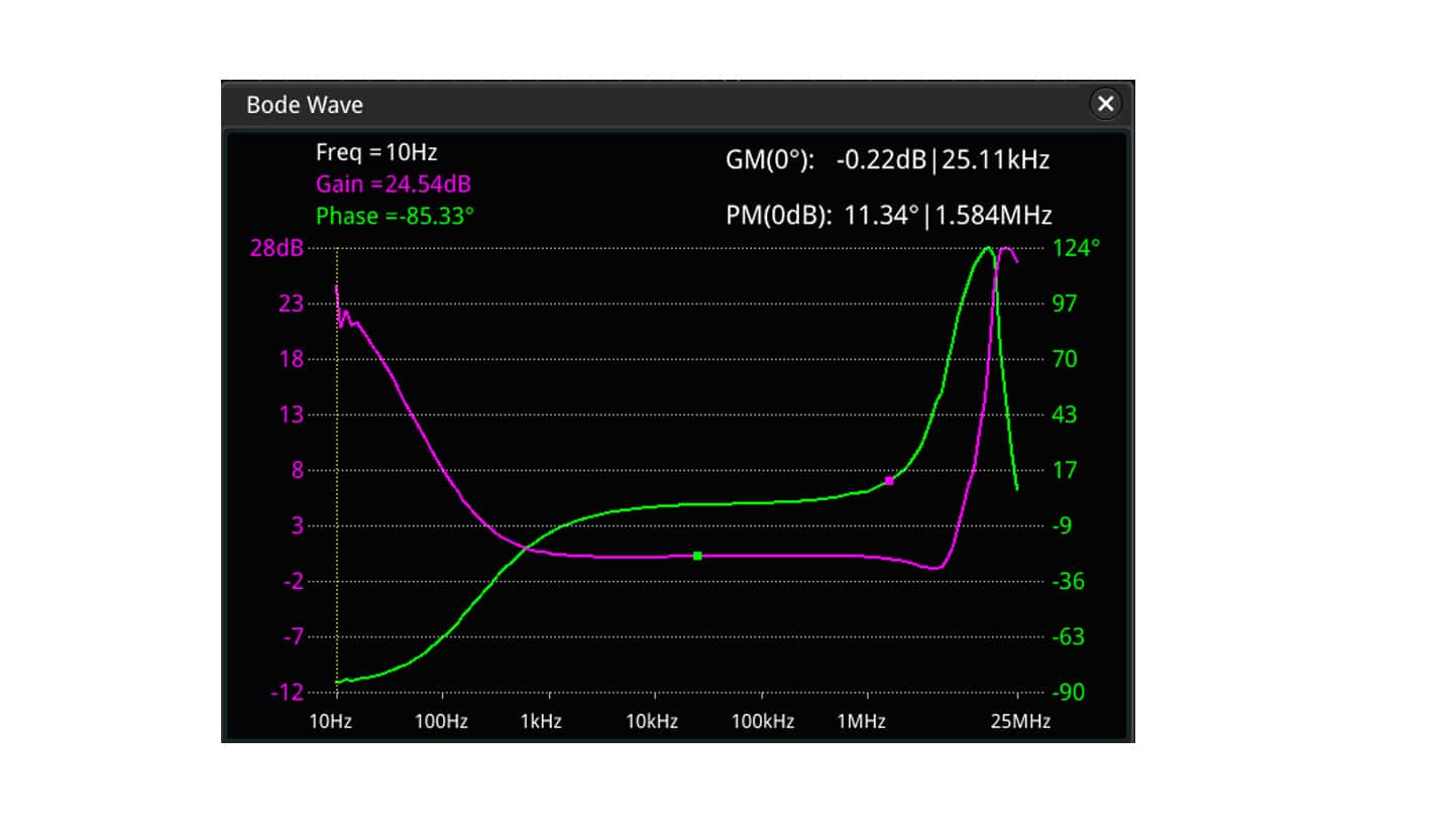
Figure 3: Measurement of PM and GM with the Bode diagram of the MSO5000.
In some circuits using amplifiers, for example, amplitudes that are too low can give an incorrect result because the output amplitude is too low to get a value of gain that can be evaluated. To do this, the input amplitude would have to be increased, which has the drawback that the frequency-dependent amplifier can saturate in another, higher frequency band and the output signal is distorted. To remedy the problem, the MSO5000 offers an amplitude variation across the frequency range. This means that a higher input amplitude could be set in the lower decades and a lower amplitude value for higher frequencies.

Figure 4. Measurement of a low pass filter with the Bode plot function on the MSO5000.
When measuring input and output voltage it is important to use the correct probe. The standard auxiliary probes of the PVP2350 version offer two different gains. To achieve a higher level of accuracy in the measurement result it is advisable to set the amplification factor to x1 for the Bode plot measurement. The bandwidth now limited to 35 MHz and the maximum voltage to be measured of 150 Vrms are sufficient for this measurement. Also, the ground connection should have a very short wire. A ground spring is included as an accessory with the probe for a very short connection to ground. With the measurement of the filter in Figure 4, the phase curve and the frequency response of the amplitude change can be seen. All points in MSO5000 can be measured separately with the cursor. These measured values can also be displayed in a table and saved as a *.csv file.
The effects of a filter can also be illustrated with the FFT built into a frequency measurement. In Figure 5 a sinusoidal signal was input to the filter of Figure 4 and measurements were taken at the output of the filter. The result is given in the frequency domain of the MSO5000 series oscilloscope. All frequency components are visible with 1 million FFT samples and display density.
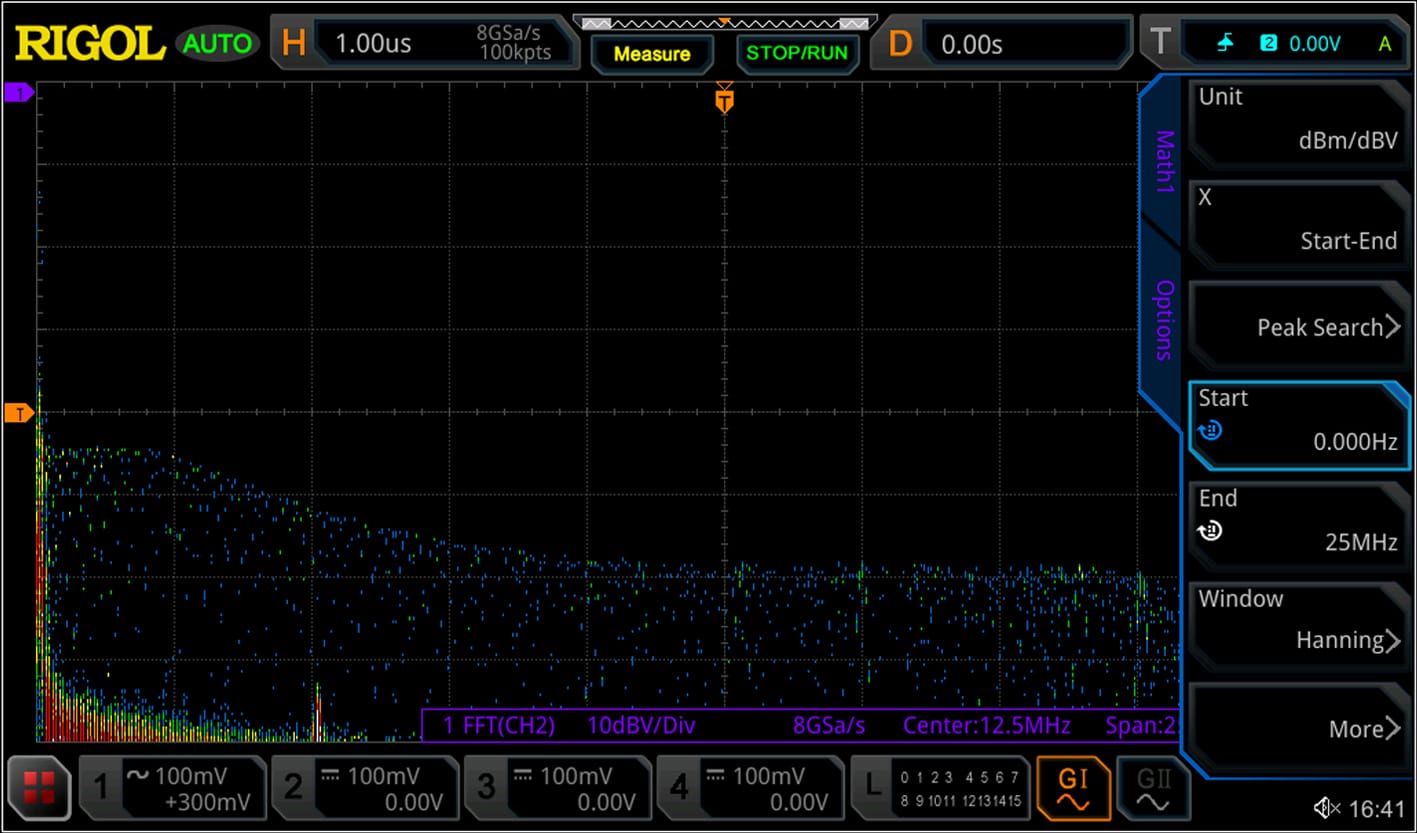
Figure 5. Frequency measurement with a swept sinusoidal signal using the MSO5000 generator.
RIGOL oscilloscopes with UltraVision II offer various standard or optional features such as zoom triggering or very high sample rate 8 GS/s bus system decoding along with very deep memory up to 200 Mpts along with the optional use of the 16 digital channels. The multiple possibilities of the oscilloscope provide an optimal solution for various applications, especially in the field of research and development, industry or education. The MSO5000 series not only offers the optimal solution for the methods and measurements described in this article, but they are powerful measurement devices with the highest levels of quality and performance at an unprecedented price. In addition to the standard probes already included, the devices also provide a wide range of current clamps, differential and high voltage probes, among many other options, all with the aim of allowing the appropriate measurement connection for each application. The detailed user manual as well as the device's menu navigation are also available in German.


